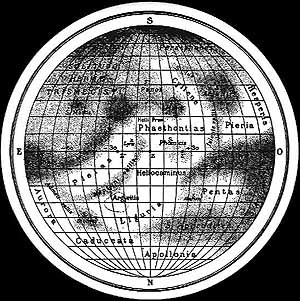
Mercury Transit on May 7, 2003 Mapping Mercury The mystery planet Mercury , the planet closest to the Sun, was well known to many ancient people. They observed it as a comparatively bright object in the evening or morning sky, close to the horizon just after sunset or before sunrise. This celestial body remained a mystery for a long time. Since it is always seen quite close to the Sun in the sky, it was mostly lost in the solar glare and often obscured by haze and dust in the Earth's atmosphere. Even the best telescopic views showed Mercury as an indistinct object, without any easily detectable surface details. It is less than 30 years ago that Mercury finally gave up many of its secrets. In 1974-75, NASA's Mariner 10 spacecraft photographed over 45 per cent of Mercury's surface . On this page, you will find information about the mapping of Mercury's surface. Early Maps of Mercury Just before he died in 1543, Nicolaus Copernicus , the famous Polish astronomer who described the heliocentric ("Copernican") system, expressed regret that he had never seen the planet Mercury with his own eyes. The first astronomer, who is known to have observed Mercury in some detail is the German astronomer Johann Hieronymus Schroeter , who lived from 1745 to 1816. He made detailed drawings of Mercury's surface features, but his sketches were not very correct. Later, straight features and lines - similar to the intriguing "Martian Canals" - were also described on Mercury by the Italian astronomer Giovanelli Schiaparelli (1835 - 1910) and also by the American astronomer Percival Lowell (1855-1916). |  | | Antoniadi's map of Mercury (ca. 1920). |
The Franco-Greek astronomer Eugenios Antoniadi (1870-1944) charted the surface of Mercury in great detail during the early 20th century. His maps were in use for almost 50 years. He looked through powerful telescopes of his time and found that the supposed Mercurian "canals" were in fact just optical illusions. It was later learned that those on Mars were not real either. In 1974-75, the NASA space probe Mariner 10 finally provided the first close-up images of Mercury. The revolutionary results of this very successful space mission forced the astronomers to redraw their earlier telescopic charts and maps. They recognized that many of the topographic features recorded until then by means of visual observations through ground-based telescopes were either non-existent or had been mapped wrongly, beacuse of the erroneous assumption that Mercury always turns the same hemisphere towards the observers on Earth. We no know that this is not the case; see the explanation about the day and night on Mercury. Thus, the exploration of Mercury's surface is based almost exclusively on information obtained by space probes. All modern maps of Mercury's surface features and our knowledge about this planet's other physical characteristics have come from this fantastic and successful mission of Mariner 10 . Nevertheless, more recent radar measurement by some of the largest radiotelescopes have also been very useful. Intricacies of planetary mapping | 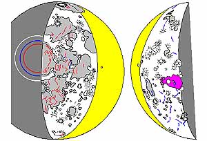 | | Provisional (draft) maps of Mercury's surface from Mariner 10 data and images. |
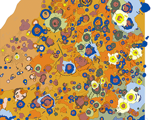
Most people have seen a globe or map of one of the other moons and planets in the solar system. It is not always appreciated how extremely difficult it is to record and chart the strange and fascinating surfaces of these other worlds. The mapping process starts with the difficult generation of the necessary images. Most spacecraft, e.g., the Pioneer and Voyager probes, passed the target planets and moons at high speeds, often at thousands of kilometers per hour. So it is a complex task to obtain good and sharp pictures or their surfaces. The on-board cameras must be pointed in the right direction and the exposure times must be sufficient short to avoid image blurring. Many probes had special cameras on-board which scanned the surfaces. The digital data are transmitted bit-by-bit back towards Earth, where they are captured by large radio antennae, e.g., the global NASA antenna system known as the Deep Space Network. Specialised computer software then turn these data into photos which constitute the basic information that serves to creating maps and globes. The next difficult task in this process is to handle various problems which are unknown in terrestrial cartography. For example, on the Earth, mountain heights are measured relative to the (mean) sea level. But the Earth is the only planet in the solar system where oceans exist which provide such a well-defined level. So which kind of elevation reference points can mapmakers then rely on when they chart the other worlds? Moreover, terrestrial maps are "tied" to accurately defined checkpoints, which are measured directly on the ground. Since long, mapmakers have selected distinct features on the terrestrial surface and have defined exactly their coordinates (geographical latitude and longitude). These "reference points" then serve to "fix" firmly the maps on the terrestrial surface. This is not so easy in the case of other planets or moons. There, the mapmakers must use a combination of measurements, including that body's accurate position in its orbit, the precise position in space of the spacecraft at the moment of the exposures and, not least, the exact pointing angle (the "line-of-sight") of the on-board camera. Moreover, it is necessary to perform a careful analysis of the geometric and optical deformation in the obtained images. In a next step, the mapmakers combine the data from several exposures by means of the method of photogrammetry, thereby "linking" the photos. The resulting charts from modern space-borne cameras will distinguish between at least 256 intensity levels. By combination of several exposures obtained in different spectral regions (i.e., through different optical filters), they may also reveal the colours of the surface material. The photomosaics obtained by images from spacecraft cameras do not provide immediate and clear information about the three-dimensional shapes; the altitudes must be deduced by additional analyses. For this, it helps to have available exposures taken at different angles of the infalling sunlight, revealing the shapes of the surface features by means of different patterns of the corresponding shadows. Airbrush maps | 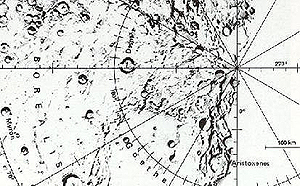 | | Airbrush map of Mercury. |
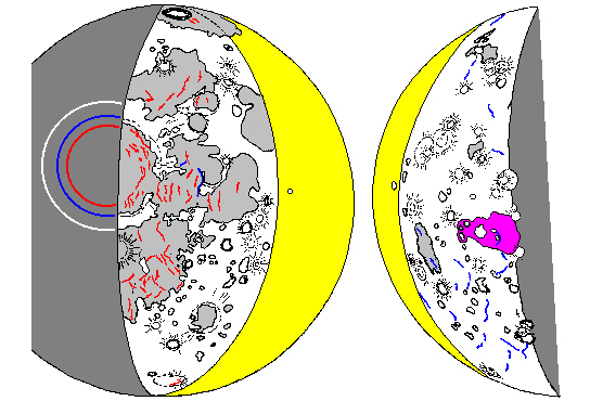
As a result of these uncertainties, maps of moons and planets are usually produced as somewhat unsharp charts. They are prepared by expert mapmakers who draw the composite pictures with a spray gun known as an "airbrush". Maps produced with this particular technique possess an amount of details that is impossible to reach in direct photos and digital cartography. Whenever possible, topographic maps are also produced, especially when this is supported by radar altimetry on-board the space probe - this has been done in the case of planet Venus. The airbrush maps are both impressive and fascinating. To produce them requires talent, a very professional handling of the spray gun and - following the careful study of the available photos - the ability to paint a picture of the imaginary or virtual surface features. Here, true artistic abilities and some measure of inspiration is needed. Mapping Mercury | 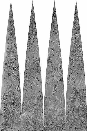 | | Mercury sectional charts - the basic tool to make a globe. |
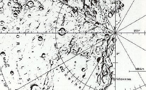
During its mission, Mariner 10 had three encounters with Mercury during which it obtained images of the surface. The first flyby took place on March 29, 1974, at an altitude of 705 km. A second encounter with Mercury occurred on September 21, 1974; this time at a distance of 47,000 km. The sunlit side of the planet and the south polar region were photographed. The third and final encounter occurred on March 16, 1975, at an altitude of only 327 kilometers and about 300 photographs were obtained. Altogether, Mariner 10 obtained about 1000 photographs of Mercury, revealing a surface riddled with craters and other interesting geological features. Now, almost three decades later, these pictures still remain our best source of information for the study of Mercury's surface. In order to facilitate the reference to a specific location or region of the planet, Mercury has been divided into fifteen quadrangles and some of the largest and most distinguishing features have been named. The quadrangles are separated and numbered according to their location, starting with H-1 at the north geographic pole and ending with H-15 at the south geographic pole. Similar systems are also used for other planets and moons with named features, and the "H" stands for Hermes ; this helps to distinguish Mercury maps and features from those on other bodies. Mercury's surface shows the following types of features: crater, albedo feature, dorsum, mons, planitia, rupes and valles . The word "albedo" is much used in astronomy and refers to the reflectivity of a surface, i.e. how bright or dark it is. Below follows some more information about these formations. | 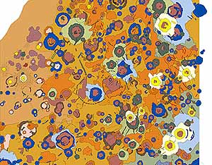 | | Geological map of Mercury craters. |
Craters : Mercurian craters have the same properties as lunar craters. The smaller craters are bowl-shaped, and with increasing size, they develop scalloped rims, central peaks, and terraces on the inner walls. The "ejecta sheets" (the material that was excavated and displaced during the impact by which a crater was formed) have a hilly, lineated texture and there are swarms of secondary impact craters from falling blocks. "Fresh" (younger) craters of all sizes have dark or bright halos and well-developed ray systems. The brightest crater is named Kuiper (after the Dutch-American astronomer Gerald Kuiper ) - it has a diameter about 60 km. Intercrater plains : Mercury's oldest surfaces are its intercrater plains - the same type of feature is also present on the Earth's Moon. These plains consist of level to gently rolling terrain that occurs between and around large craters. They predate the heavily cratered terrain, and presumably cover many of the earliest craters and basins of Mercury. Basins: At least 15 ancient basins have been identified on Mercury. Tolstoj is a true multi-ring basin, displaying at least two, and possibly as many as four, concentric rings. Beethoven has only one subdued, massif-like rim that measures 625 km in diameter. The Caloris Basin is defined by a ring of mountains, 1300 km in diameter. Smooth plains : Widespread areas on Mercury are covered by relatively flat, sparsely cratered plains. These plains are similar to the "mare" ("seas") on the Moon; they are most strikingly present in a broad annulus around the Caloris basin. Names of Mercury features | 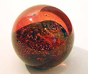 | | A Mercury globe. |
Features on the surface of any planet or moon in the solar system are named in compliance with the rules and conventions set by the International Astronomical Union (IAU) since 1919. It is a fundamental principle to exclude political, religious and living persons. Unique themes are set for each type of feature on individual planets or moons to which any new name must adhere. On Mercury, craters are named after famous artists, painters, authors, and musicians (who have been dead for at least three years); "planitiae" are named after the names for Mercury (referring to either the planet or the god) in other languages; scarps , also known as "rupes" , are named after vessels of famous discoverers, for example Discovery , the ship of Captain Cook ; valles are named after radio telescope facilities; and the only montes known on the planet are named Caloris , from the Latin word for "hot". At the beginning of planetary exploration, it usually took several years to set up a naming system and to assign official names to the discovered topographic features. To speed up this process, the IAU now collects suitable names in databanks in advance and then give them to the features soon after discovery. For more information on how features on the surfaces of planets and moons are named, visit this site: http://planetarynames.wr.usgs.gov |
|
|
| | |